

To tune a model of the Black Death, we need one number that says how badly a run disagrees with the historical record. The lower the number, the better the run. This article explains how we build it.

Comparing to Priest Deaths
Few records indicate when ordinary people died between 1348 and 1350. Priests are an exception. When a parish priest died, the bishop had to fill the post, and his registers note the date. We have about 4,900 such deaths, spread across some 3,400 manors in England. Priests are not a perfect sample: they were adult men who visited the sick, so their deaths may not track the wider population. They are, though, the largest set of dated, placed deaths we have.
The model records every simulated death with a day and a manor. So for each priest we ask: could this date have come from the model’s deaths at the same place?
Scoring against one priest death
At a given manor, the model might produce a few hundred deaths scattered over many days. It may come in several waves or just one – we can’t know a priori. We need a statistical method to turn this jumble of deaths outputted from the model and compare it to a priest death in the area. For this, we use a method called conformal prediction.
We want to know how likely the model thinks a death is on any one day. First, we smooth the dates to remove some of the noise of the model. We swap each simulated death for a small bell-shaped bump centred on its day, about a day and a half wide, and add the bumps together. Scaled so the area beneath it is one, the result is a curve, , whose height gives the share of deaths the model expects on day .

The idea is that deaths occurring near a peak in are common, whereas deaths occurring when is very small are unusual. To quantify this, each simulated death gets an “oddness” score,
which is small for days near the peak, where deaths are common, and large for days in the tails, where deaths are rare.
The log keeps the numbers easy to handle: each extra point of oddness means the date is nearly three times less likely. We score every simulated death at its own date, and these scores become the yardstick. A priest death is scored from the same curve, at the date in the bishop’s register.
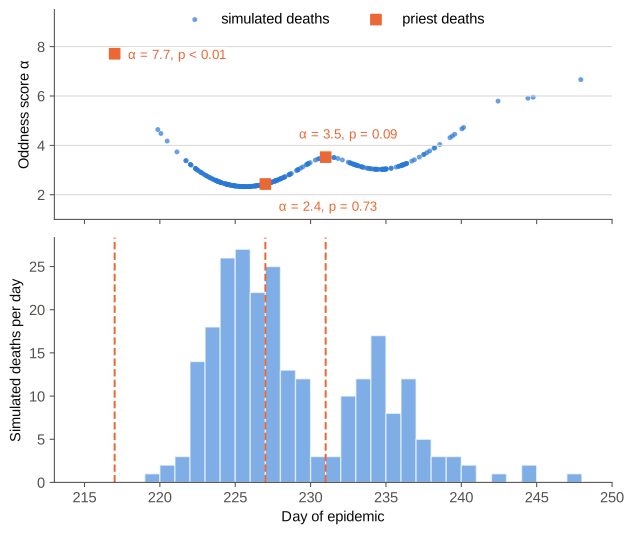
A priest death gets the same score from its own date. Its p-value is the share of simulated deaths that are at least as odd:
where is the number of simulated deaths at that manor. A priest who died at the height of the local outbreak scores close to 1, because nearly every simulated death is odder than theirs. A priest who died months after the model’s outbreak had burnt out scores close to 0. The extra one keeps above zero.

Figure 3 shows the scores of three priests at the same manor. The one who died on day 227, at the main peak, gets a low score. The one on day 231, in the lull between two waves, scores higher, and the one on day 217, before the model’s outbreak began, higher still. Only the oddness counts, not which side of a peak the date falls.
To turn a score into a p-value, we line up the scores of all simulated deaths at the manor and count those at least as odd as the priest’s. For the priest at the peak, 176 of 245 count and p is 0.72. Only 21 count for the priest in the lull, giving 0.09, and none for the early priest, giving less than 0.01. In practice we soften the sharp count, so that a wee change to the model gives a small change in the score, as the fitting software needs.
From many deaths to one number
We combine the p-values of all priest deaths into a single error
where is the p-values for each priest death . Taking the log means one wildly unlikely death, with p near zero, adds a large penalty. The model cannot hide a manor it gets badly wrong behind many it gets right. Statisticians know this as Fisher’s method.
The error is lowest when every priest death falls at its manor’s peak, with near 1. So it rewards a model whose busiest weeks line up with the priest deaths.
What we aim for
Even a perfect model would not reach that lowest error. If priest deaths came from the model itself, their p-values would land anywhere between 0 and 1 with equal chance, and average 0.5. We test this by scoring fresh simulated deaths against their own manor’s curve. The result is close to flat, with a mean near 0.5.
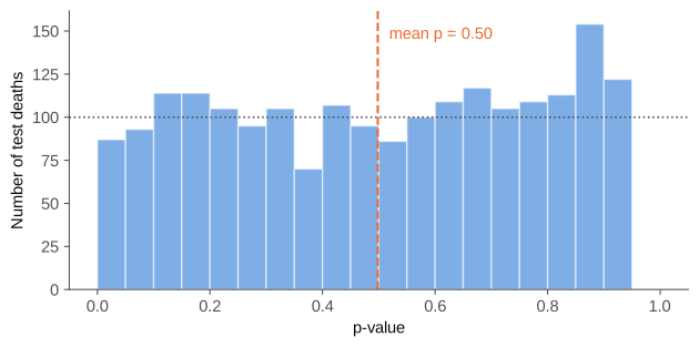
This gives a second, gentler test of a fitted model. If its priest p-values also spread evenly, the model is as consistent with the record as chance allows. If they bunch near 0, it suggests that the priest deaths are consistently ‘odd’ compared to the model outputs, so the model and the priest data do not conform well.
Next step: Manor court rolls
Manor courts met every few weeks and often recorded the tenants who had died since the last sitting. These give counts of deaths in a window rather than single dates, and we plan to add them to the error. If the previous sitting fell within about 45 days, the recorded count is an exact target. If the gap is longer, or there is no earlier roll, rolls may be lost, so the count is only a minimum. An exact target is penalised for missing either way, a minimum only when the model predicts too few deaths.
